
Rearranging embedded lists with purrr
Honestly, I am not even sure what to title this post. I can’t remember what I googled that eventually took me to a website that answered my question, but I think it was something a long the lines of “re-level embedded list R” maybe? Anyways… the nifty trick that I eventually came accross that does exactly what I want is probably worth a blog post…
Let’s say that I have a list of utilization distribution objects (each calculated using locations collected during a different year) embedded in a list of of different individuals (so, the list structure is Individual > Year > Object). But what I want is a list of UDs for each individual, embedded in each year (so, Year > Individual > Object). To put it visually, I want to go from this, to that…
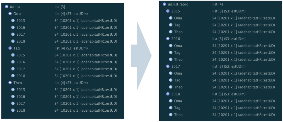
(left) this, and (right) that
A simple example
I’ll generate some simple data to work with. The data will have 5 variables:
- Individual ID
- Individual colour
- Year
- X position
- Y position
I’m just using a regular numeric variable for X and Y location values; these can be likened to the coordinate values in a projected coordinate system, such as the Universal Transverse Mercator (UTM) coordinate system.
library(adehabitatHR)
library(viridis)
set.seed(100)

#generate random data for 3 different individuals, assign year randomly
years <- c("2015", "2016", "2017", "2018")

data <- data.frame(rbind(cbind(X = rnorm(300, 25, 4), Y = rnorm(300, 25, 7),
                               Year = sample(years, 300, replace = TRUE), Ind = "Oma"),
                         cbind(X = rnorm(300, 30, 6), Y = rnorm(300, 30, 3),
                               Year = sample(years, 300, replace = TRUE), Ind =  "Tag"),
                         cbind(X = rnorm(300, 50, 2), Y = rnorm(300, 50, 10),
                               Year = sample(years, 300, replace = TRUE), Ind = "Theo")))

# tidy it up a bit and sort by individual then by year
str(data)
## 'data.frame':    900 obs. of  4 variables:
##  $ X   : Factor w/ 900 levels "12.9167428039385",..: 116 234 203 376 229 276 103 342 74 143 ...
##  $ Y   : Factor w/ 900 levels "1.75452456443001",..: 8 45 38 70 257 489 187 255 7 304 ...
##  $ Year: Factor w/ 4 levels "2015","2016",..: 4 4 2 2 1 2 4 3 4 4 ...
##  $ Ind : Factor w/ 3 levels "Oma","Tag","Theo": 1 1 1 1 1 1 1 1 1 1 ...

data$X <- as.numeric(as.character(data$X)) #make the numbers numeric
data$Y <- as.numeric(as.character(data$Y)) #make the numbers numeric
data <- data[order(data$Ind, data$Year), ] #order the rows by Ind then by Year

summary(data) #look at a summary of the data
##        X               Y            Year       Ind
##  Min.   :12.92   Min.   : 1.755   2015:222   Oma :300
##  1st Qu.:25.27   1st Qu.:26.883   2016:208   Tag :300
##  Median :31.47   Median :31.240   2017:235   Theo:300
##  Mean   :35.17   Mean   :34.885   2018:235
##  3rd Qu.:48.47   3rd Qu.:44.235
##  Max.   :56.33   Max.   :77.269

# add some colours to make things easier to visualize
colstart <- viridis(3)
data$IndCol <- ifelse(data$Ind == "Oma", colstart[1],
                      ifelse(data$Ind == "Tag", colstart[2], colstart[3]))


# take a look at these points
plot(data$X, data$Y,
     asp =1,
     pch = 16,
     col = data$IndCol)
legend("topleft", legend = c("Oma", "Tag", "Theo"), pch = 16, col = colstart)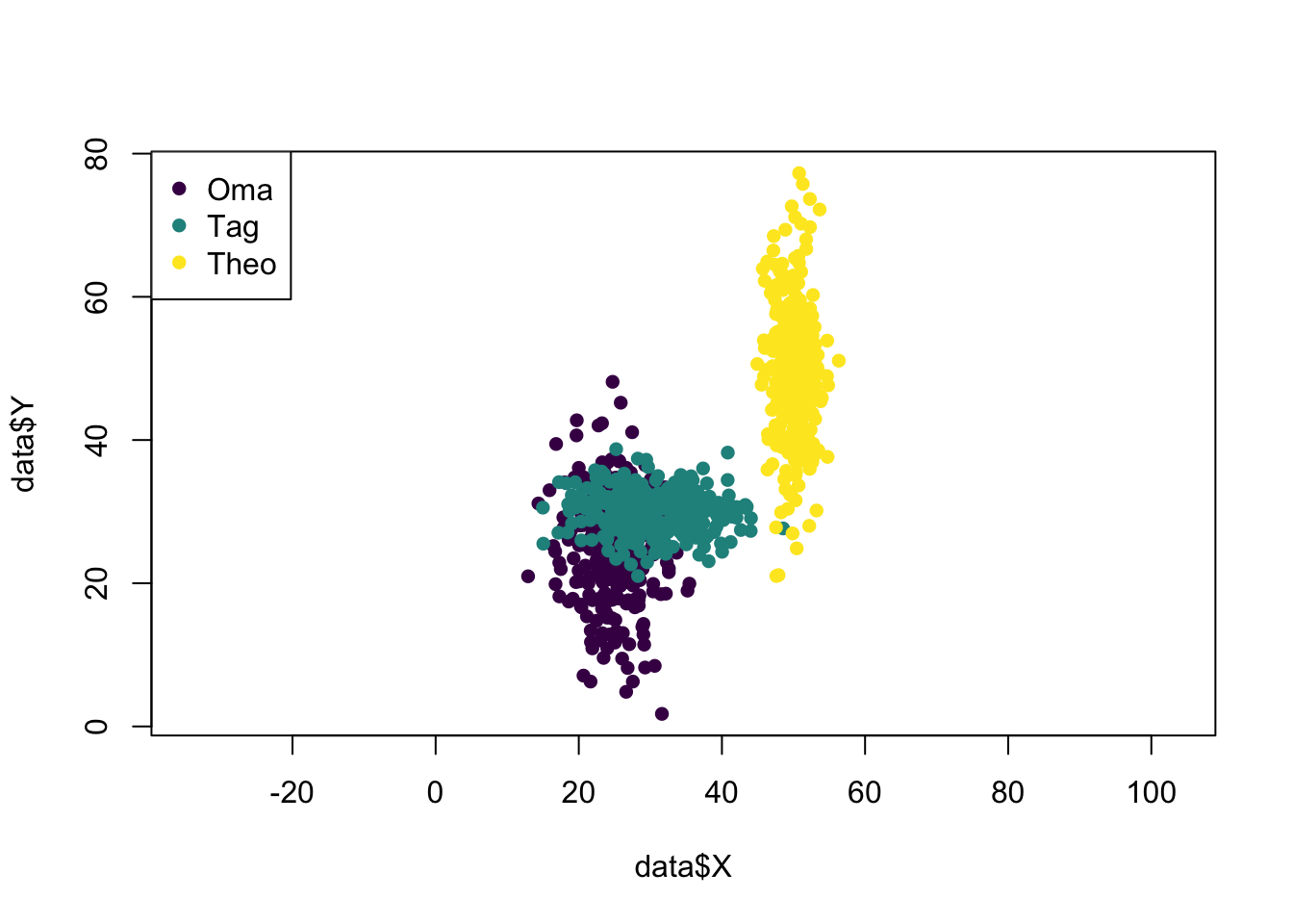
# add an increasingly large X or Y shift to each individual over 'time'
# (just to make it more interesting)
data$X <- c(data$X[1:300] + seq(from = 0, to = 15, length.out = 300), #give Oma a postitive X shift
            data$X[301:600], #leave Tag's X coords alone
            data$X[601:900] - seq(from = 0, to = 25, length.out = 300)) #give Theo a negative X shift

data$Y <- c(data$Y[1:300], #leave Oma's Y coords alone
            data$Y[301:600] + seq(from = 0, to = 20, length.out = 300), #give Tag a positive Y shift
            data$Y[601:900]) #leave Theo's Y coords alone

# now plot this new data, with the shift
plot(data$X, data$Y,
     asp =1,
     pch = 16,
     col = data$IndCol)
legend("topleft", legend = c("Oma", "Tag", "Theo"), pch = 16, col = colstart)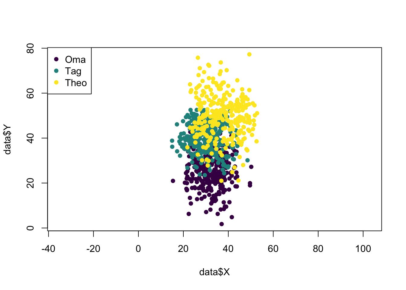
# now let's break the data in a list, with each individual as one item in the list
data.lsted <- split(data, data$Ind) #split it
data.lsted <- lapply(data.lsted, droplevels) #drop the other individual factor
                                          #levels from each dataframe in the list
Now that we have the data, listed by individual, I’ll go through the steps to calculate the home ranges (using the adehabitatHR package), of each individual for each year…
# turn each individual's dataframe into a SpatialPointsDataFrame with the year as the data
spdf <- lapply(data.lsted, function(x) SpatialPointsDataFrame(coords = x[c("X", "Y")],
                                                                           data = x["Year"]))

# make a grid in which to calculate the UDs
grid.xy <- expand.grid(x=seq(0, 100, by=1), y=seq(0, 100, by=1))
grid.sp <- SpatialPoints(grid.xy)
gridded(grid.sp) <- TRUE

# calculate the kernel UD of each individual for each year (this function will automatically
# calculate one UD for each factor level of the data column in the SpatialPointsDataFrame, i.e. in
# this case, one UD for each year)
ud <- lapply(spdf, function(x) kernelUD(x, h="href", grid=grid.sp, kern="bivnorm"))

# get the 90% UD outline for each individual for each year
vt <- lapply(ud, function(x) getverticeshr(x, percent = 90))

# now plot it (3 plots with a legend underneath)
# sort out plotting layout
m <- matrix(c(1,2,3,4,4,4), nrow = 2, ncol = 3, byrow = TRUE)
layout(m, heights = c(0.9, 0.1))

# plot the ranges
par(mar=c(5.1,4.1,4.1,2.1))
for (i in 1:3) {
  plot(vt[[i]],
       axes = T,
       xlim = c(0, 60), ylim = c(0, 80),
       lwd = 3,
       border = viridis(4),
       main = names(vt)[i])
}
# plot the legend
par(mar=c(0,0,0,0))
plot(1, type = "n", axes=FALSE, xlab="", ylab="")
legend("top", inset = 0, legend = c("2015", "2016", "2017", "2018"),
                       lty =1, lwd =3,
                       col = viridis(4),
                       horiz = TRUE)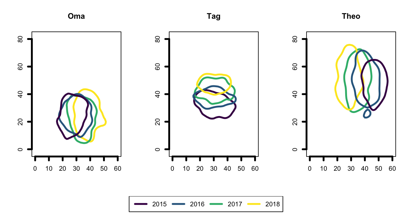
Now, time to go from this to that; We have a list of individuals, with a sublist of years’ UD objects. I want to switch up the nested structure; so I want a list of years, each with a sublist of individuals’ UDs.
I’ll do this using the map function from the purrr package.[^1] The map function works like a base apply function. Here, the ‘function’ I’ll apply is [[ (basically “pull”) and I’ll apply it to each year’s UD, one year at a time.
library(purrr)

ud.reorg <- list() #initialize the output list

for (i in seq_along(years)) { #for each year
  ud.reorg[[years[i]]] <- map(ud, `[[`, years[i]) #HERE IS THE NIFTY TRICK PART!
                                                        #(see text below)
  class(ud.reorg[[years[i]]]) <- "estUDm" #join these new sublists into `estUDm` objects
                                            #(allows for application of functions such as
                                            #getverticeshr and overlap)
}

# get the 90% UD outline for each year for each individual
vt.reorg <- lapply(ud.reorg, function(x) getverticeshr(x, percent = 90))

# now plot it (4 plots with a legend underneath)
# sort out plotting layout
m <- matrix(c(1,2,3,4,5,5,5,5), nrow = 2, ncol = 4, byrow = TRUE)
layout(m, heights = c(0.9, 0.1))

# plot the ranges
par(mar=c(5.1,4.1,4.1,2.1))
for (i in 1:4) {
  plot(vt.reorg[[i]],
       axes = T,
       xlim = c(0, 60), ylim = c(0, 80),
       lwd = 3,
       border = viridis(3),
       main = names(vt.reorg)[i])
}

# plot the legend
par(mar=c(0,0,0,0))
plot(1, type = "n", axes=FALSE, xlab="", ylab="")
legend("top", inset = 0, legend = c("Oma", "Tag", "Theo"),
                       lty =1, lwd =3,
                       col = viridis(3),
horiz = TRUE) 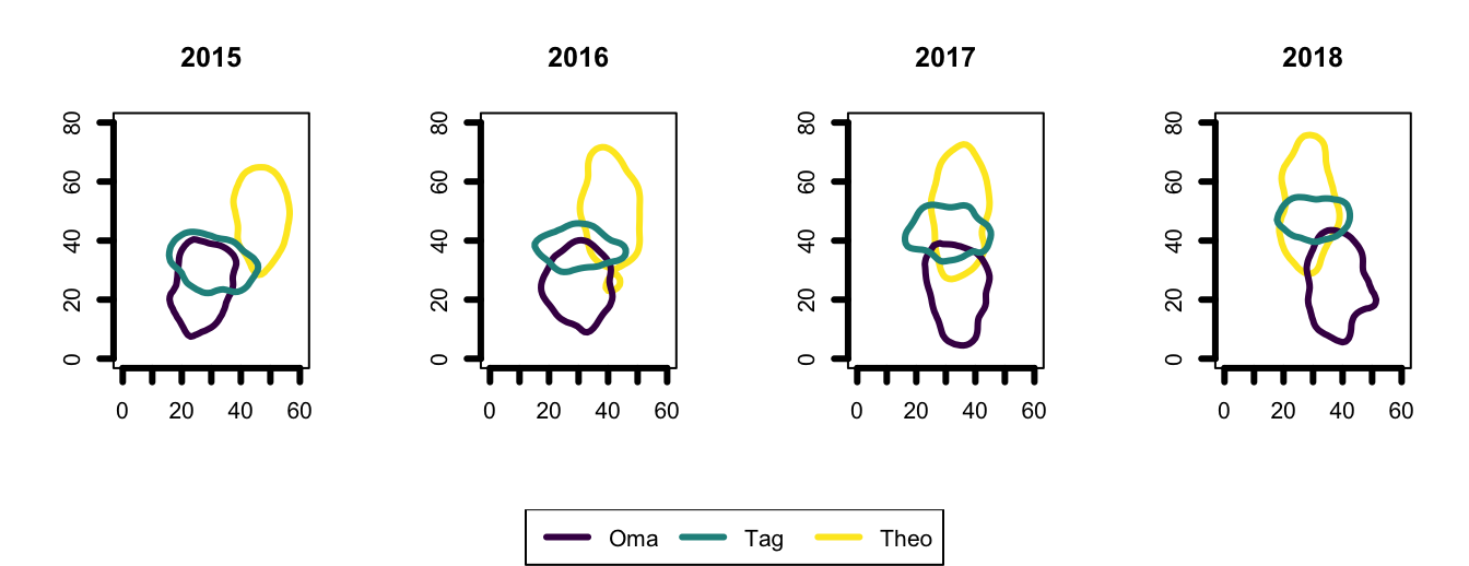
So, the nifty trick part is:
ud.reorg[[years[i]]] <- map(ud, `[[`, years[i])Let me try to explain what is happening here:
With every iteration of the loop (i.e. for each factor level of years), the code:
1) initializes a sublist for that year (years[i]),
2) uses the map function to pull out ([[) the objects named with that year (years[i]) from the original data (ud),
3) sticks these objects into the new sublist (<-). ((Note that the map function automatically renames the pulled objects in new sublist, giving them the name of their original sublist, in this case, the name of each individual.))
The last line of code in the loop (class(ud.reorg[[years[i]]]) <- "estUDm") is specific to these particular UD objects: I want the UD objects in each sublist to be grouped as a complete estUDm object, which will allow for calculations such as overlap between UDs, etc.
More purrr::map magic
Another purrr function that I wish I’d known about years ago is the map2 function. It works like the map function (like a base apply function) but it takes two objects as inputs, which can both be used in the applied function. The map2 function will “line up” the two objects and perform the function between parallel elements. So, for example….
#load the package
library(purrr)

#make a list that has embedded lists
mylist <- list(a = list(9, 12, 15),
             b = list(12),
             c = list(15, 20))

#make another list with the exact same structure and number of objects
foo <- list(a = list(3, 4, 5),
             b = list(3),
             c = list(13, 5))
So now, let’s say that I want to divide the objects (in this case, just numbers) in mylist by their corresponding objects (numbers) in foo. For this, I can use the map2 function…
#for just one of the embedded lists in mylist and foo
out1 <- map2(mylist[["a"]], foo[["a"]], function(x, y) x/y)
out1
## [[1]]
## [1] 3
##
## [[2]]
## [1] 3
##
## [[3]]
## [1] 3

#to apply the map2 function to all of the lists embedded in mylist and foo
out2 <- map2(mylist, foo, map2, function(x, y) x/y)
out2
## $a
## $a[[1]]
## [1] 3
##
## $a[[2]]
## [1] 3
##
## $a[[3]]
## [1] 3
##
##
## $b
## $b[[1]]
## [1] 4
##
##
## $c
## $c[[1]]
## [1] 1.153846
##
## $c[[2]]
## [1] 4

#an example where it's easier to see...
out3 <- map2(mylist, foo, map2, function(x, y) paste(x, "/", y, "=", x/y))
out3
## $a
## $a[[1]]
## [1] "9 / 3 = 3"
##
## $a[[2]]
## [1] "12 / 4 = 3"
##
## $a[[3]]
## [1] "15 / 5 = 3"
##
##
## $b
## $b[[1]]
## [1] "12 / 3 = 4"
##
##
## $c
## $c[[1]]
## [1] "15 / 13 = 1.15384615384615"
##
## $c[[2]]
## [1] "20 / 5 = 4"
Super great right?
So much more to learn
This purrr package kinda blows my mind - I feel like, lately, every time I’ve come accross a crazy simple hack for a complex list-related problem, it been something from the purrr package. I’ve only just scratched the surface in terms of its many capabilities. Find out more info about this package, including a cheat sheet, here. I also really like this tutorial. And if you have any tips, tricks, suggestions, or links of your own on this topic, please post them in the comments!