
Minimizing error in animal tracks
Day Journey Length (or “DJL”), also known as “daily travel distance,” “daily path length,” and other terms, is the cumulative euclidian distance that something (in my case, an orangutan) travels over the course of a day. This is a common measure used in all types of animal ecology and animal behaviour research, as it is a simple measure to characterize movement patterns, quantify an animal’s interaction with its habitat, and it is one indicator of energy expenditure. Of course, unless the location data are collected continuously and with perfect accuracy (which is generally impossible with GPS unit/tag), then there is inevitably at least some estimation involved in this measure. That said, it’s important to at least be sure that, where there are sources of error, these are unbiased and randomly distributed throughout the data. This, however, was not the case for orangutan DJLs at my field site…
My DJL overestimation situation
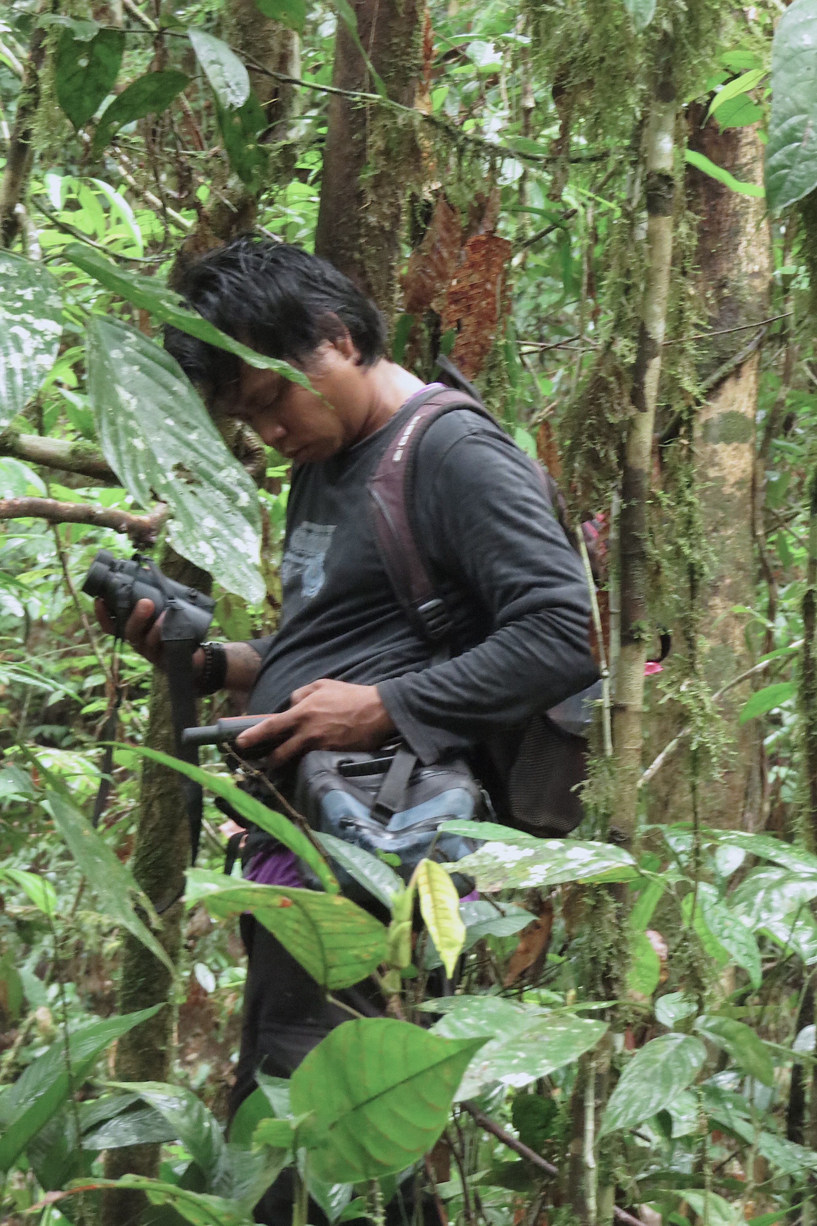
I noticed a while back that my DJLs of unhabituated orangutans who hardly moved at all during a day were waaaay too long. I knew - from being there, waiting under the tree - that an orangutan had moved no more than 30 meters all day, and yet I was getting DJLs of over 400 meters. Basically, the less an orangutan moved during a day, the more error there seemed to be in the cumulative length of its day-long track. This error is mostly caused by the GPS bouncing around and having an imprecise fix (more severe in areas with low satellite coverage, varied terrain, and a dense canopy - all of which applied to my field site), but some error can also be attributed to the observer who is actually carrying the GPS unit (we can’t tag wild orangutans, so the location data we collect for them is on hand-held units) - moving around under the tree to get a better view of the orangutan, go pee, etc etc.
Furthermore, every once in a while, the GPS unit seemed to just crap out completely - losing it’s satellite reception - and take a fix way way off course. I noticed these types of errors when I was looking specifically at step lengths between 30-minute points, and finding outliers that were way beyond the distance that an orangutan would ever (under normal circumstances) move in just half an hour.
I did a lot of research and couldn’t find much info about ‘smoothing out’ this GPS error, so I decided just to write some functions for myself. If you’re reading this, and you have some idea of how other researchers and movement ecologists handle this issue - please let me know!!! Also, if you have suggestions that you think would improve my methods, get in touch! (comments, or email me! alie@aliesdataspace.com)
So, to set it up, here is the problem. Below are 3 orangutan day tracks, from nest to nest. The DJL, in meters, is in the title of each panel (also notice the scales in the bottom right corners - each one shows 10 meters). Each track starts at the blue dot and ends at the red dot, and each track (each follow of each orangutan, each day) has a unique identifying follow number.
(Note: I’m just learning to use the tidyverse, sf, and tmap libraries. I’ll show all of my code here, even for basic data set up / plotting - just incase anybody else is wrestling with these things, and/or has any feedback for me.)
#load needed packages
library(tidyverse)
library(sf)
library(tmap)

#check out the data
str(gps)
## 'data.frame':    68 obs. of  6 variables:
##  $ FolNum  : int  19 19 19 19 19 19 19 19 19 19 ...
##  $ Focal   : Factor w/ 2 levels "Pi","Roger": 2 2 2 2 2 2 2 2 2 2 ...
##  $ PtType  : Factor w/ 5 levels "FIND","LOST",..: 3 5 5 5 5 5 5 5 5 5 ...
##  $ DateTime: POSIXct, format: "2014-07-13 05:57:00" "2014-07-13 06:00:00" ...
##  $ X       : num  474432 474428 474449 474440 474422 ...
##  $ Y       : num  172843 172832 172827 172823 172831 ...
summary(gps)
##      FolNum         Focal          PtType      DateTime
##  Min.   : 19.00   Pi   :40   FIND     : 1   Min.   :2014-07-13 05:57:00
##  1st Qu.: 19.00   Roger:28   LOST     : 1   1st Qu.:2014-07-13 13:52:30
##  Median : 82.00              MORNNEST : 2   Median :2015-10-03 13:15:00
##  Mean   : 62.82              NIGHTNEST: 2   Mean   :2015-04-14 23:19:01
##  3rd Qu.:102.00              RANGE    :62   3rd Qu.:2015-11-09 08:07:30
##  Max.   :102.00                             Max.   :2015-11-09 16:07:00
##        X                Y
##  Min.   :474418   Min.   :172600
##  1st Qu.:474429   1st Qu.:172831
##  Median :474496   Median :173203
##  Mean   :474551   Mean   :173335
##  3rd Qu.:474604   3rd Qu.:173977
##  Max.   :474873   Max.   :174284


#make an sf points object - use X and Y columns to build the coordinates
pts_sf <- gps %>%
  st_as_sf(coords = c("X", "Y"),
           crs = "+proj=utm +zone=50 +north +ellps=WGS84 +datum=WGS84 +units=m +no_defs")

#make 3 sf line objects - one for each focal follow (ie group by follow number)
path_sf <- pts_sf %>%
  group_by(FolNum) %>%
  summarize(ID = Focal[1],
            StTime = min(DateTime),
            EndTime = max(DateTime),
            do_union = FALSE) %>% #keeps the points in the correct order
  st_cast("LINESTRING")

#calculate the length of each line, ie the DJL, rounded to the nearest meter
path_sf$DJL <- round(st_length(path_sf))

#plot these 3 paths
tmap_style("white")

tm_shape(subset(pts_sf, PtType == "RANGE")) + #plot the half-hour points
  tm_dots(size = 0.3, col = "black") +
  tm_shape(subset(pts_sf, PtType == "MORNNEST" | PtType == "FIND")) + #plot the start points
  tm_dots(size=0.5, col = "blue") +
  tm_shape(subset(pts_sf, PtType == "NIGHTNEST" | PtType == "LOST")) + #plot the end points
  tm_dots(size=0.5, col = "red") +
  tm_shape(path_sf) + #plot the path lines
  tm_lines(lwd = 1.7) +
  tm_facets(by = "FolNum") + #one map per follow
  tm_scale_bar(breaks = c(0,0.01)) + #add a scale bar to each map
  tm_compass() + #add a little North arrow
tm_layout(panel.labels=paste("Follow Number", path_sf$FolNum, ";", path_sf$DJL, "meters")) 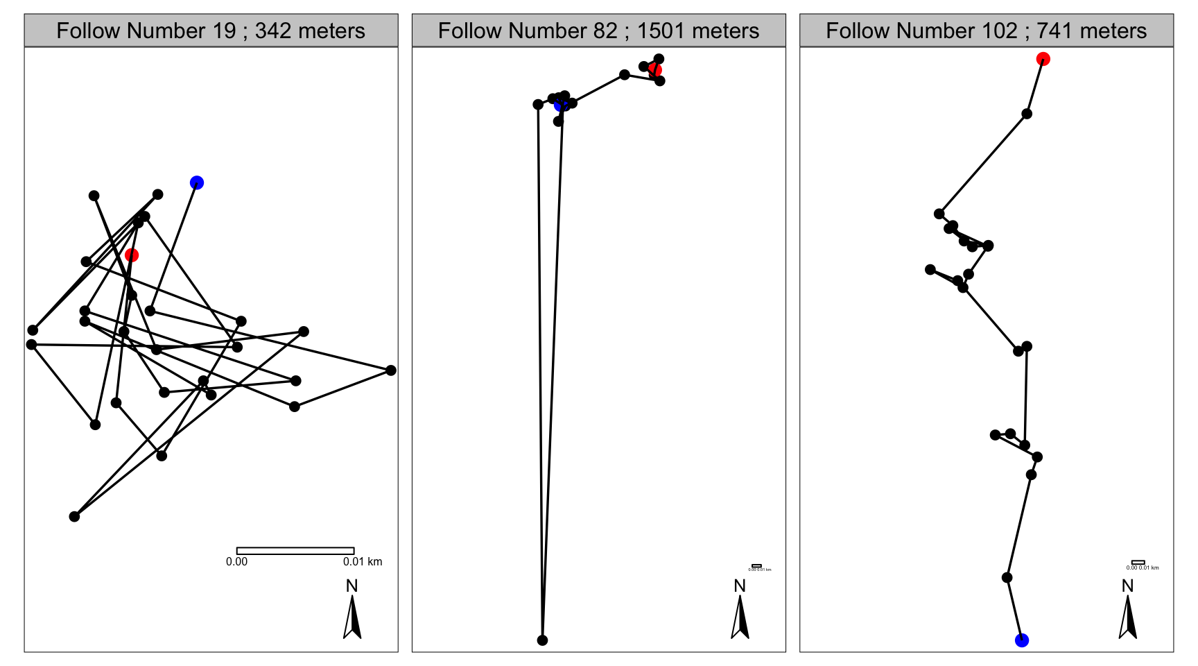
So, the issue here is: I know (from actually following these orangutans, and also just from looking at these tracks) that these DJLs are not very accurate - especially the first and second one. During follow number 19, Roger never left one single large dipterocarp tree all day. While he did move around a bit in that tree, the track made by that day’s GPS points is not an accurate representation of his movements at all - it is my movements (moving around under the tree to get a better view of him) + a hefty dose of basic GPS error (this is a really steep and hilly area with dense tree cover). Zero meters would actually be a much more accurate measure of Roger’s DJL that day. Arguably even worse, is follow number 82 - this is clearly a case of the GPS unit just totally losing its satellite reception and getting a fix way off course. I know that during this follow, Pi travelled about 200-300 meters that day, which - if we get rid of that one point that is way too far south, is probably about what her track would be. The last follow isn’t nearly as bad: during follow number 102, Pi probably travelled at least 650 meters. There is a bit of error here, probably around feeding trees (ie. places where she stopped), but overall, this path looks mostly ok. So I think these follows are good examples of what the different types of error can look like, and how it’s generally worse for follows with less directional travel.
The basic problems
So there are essentially two problems here:
Problem 1) Messy ‘stops’ - when the track actually shouldn’t be moving, but instead is jumping around back and forth, randomly. All 3 examples have a bit of this, but follow number 19 is especially bad.
Problem 2) Massive ‘jumps’ - when the GPS gets a fix that is way farther than a plausible step distance for the animal. Follow number 82 has this.
The basic solutions
I wrote two functions that I’ve used to deal with these different problems. Both functions require the coordinates to be projected (ie. X and Y, on a flat 2D surface) and just as two columns in a simple data frame (not spatially explicit objects such as sp, move, or sf objects). No points are deleted in either of these functions - although it will look like fewer points on the maps, because points get averaged out and all piled on top of each other.
Note that I wrote these functions at different times so the styles are a bit different. I’ve tried to clean up the commenting a bit here, but I’m also trying to resist the temptation to work on them and totally clean up the formatting, because I don’t really have time, and I know if I start, I’ll go down a dark path that ends somewhere with me hiding under my desk, crying about turning angles. So I’m just posting these as they are on my computer, right now, and I hope that’s ok.
Messy Stops
This first function deals with Problem 1, messy stops. It takes 4 arguments:
- df - the data frame in which the data are stored
- Xorg and Yorg - the names or numeric indices of the columns in df where the X and y coordinates are stored
- stopER - the length of the expected error, or the maximum distance that should be considered “error” (more about this below)
This whole function returns two new columns, called Xadj and Yadj, with adjusted points where necessary (and the same point coordinates as before where no adjustment was applied).
average_messy_stops <- function(df, Xorg, Yorg, stopER) {
  if (nrow(df) > 2) { ## There need to be at least 3 locations for all following...

    # set up the vars for the loops and turning fcns
    df[,"Xadj"] <- df[, Xorg] # copy X's into adjusted col
    df[,"Yadj"] <- df[, Yorg] # copy Y's into adjusted col

    # PRE-LOOP ---------- checking for 'bad starts' (i.e. imprecise stop right at beginning)
    k <- 2 # reach ahead to this point
    m <- 2 # index in storage vectors
    Xstorage <- (df[1, "Xadj"]) # begin storage vector with first point
    Ystorage <- (df[1, "Yadj"]) # begin storage vector with first point
    # this while loop reaches forwards and collects all points within the stopER radius
    while (k <= (nrow(df)) && # from the second to the last point
           (sqrt( ((df[1, "Xadj"] - df[k, "Xadj"])^2) + ((df[1, "Yadj"] - df[k, "Yadj"])^2) ) < stopER)) {
      # while pt k is still within stopER radius of first point
      Xstorage[m] <- df[k, "Xadj"]
      Ystorage[m] <- df[k, "Yadj"]
      m <- m+1
      k <- k+1
    }
    if (length(Xstorage) >= 2) {
      df[1:(k-1), "Xadj"] <- mean(Xstorage) #average out all the X vals, put in the adjusted column
      df[1:(k-1), "Yadj"] <- mean(Ystorage)  #average out all the Y vals, put in the adjusted column
    }
    rm(k, m, Xstorage, Ystorage)
    # Pre-loop ----------

    # POST-LOOP ---------- checking for 'messy ends' (i.e. imprecise stop right at end)
    k <- 1 # reach back this many points
    m <- 2 # index in storage vectors
    Xstorage <- (df[nrow(df), "Xadj"]) # begin storage vector with first point
    Ystorage <- (df[nrow(df), "Yadj"]) # begin storage vector with first point
    # this while loop reaches back and collects all points within the stopER radius
    while ( (k < nrow(df)) && # from the second to the last point
           (sqrt( ((df[nrow(df), "Xadj"] - df[(nrow(df)-k), "Xadj"])^2) + ((df[nrow(df), "Yadj"] - df[(nrow(df)-k), "Yadj"])^2) ) < stopER ) ) {
      # while pt k is still within stopER radius of first point
      Xstorage[m] <- df[(nrow(df)-k), "Xadj"]
      Ystorage[m] <- df[(nrow(df)-k), "Yadj"]
      m <- m+1
      k <- k+1
    }
    if (length(Xstorage) >= 2) {
      df[nrow(df):(nrow(df)-k+1), "Xadj"] <- mean(Xstorage) #average out all the X vals, put in the adjusted column
      df[nrow(df):(nrow(df)-k+1), "Yadj"] <- mean(Ystorage)  #average out all the Y vals, put in the adjusted column
    }
    rm(k, m, Xstorage, Ystorage)
    # Post-loop ----------

    # MAIN LOOP ---------- averaging out 'messy stops' throughout the track
    j <- 1 # current point
    for (j in 1:nrow(df)) {
      k <- j+1 # next point
      m <- 2 # next position index for storing XY coords in the storage vectors
      Xstorage <- df[j, "Xadj"] # store the current X coord
      Ystorage <- df[j, "Yadj"] # store the current Y coord
      # this while loop reaches forward from point j to point k (which counts up) and stores pt k's XY coords in vectors, as long as 2 criteria are met:
      while (k <= (nrow(df)) &&
             (sqrt( ((df[j, "Xadj"] - df[k, "Xadj"])^2) + ((df[j, "Yadj"] - df[k, "Yadj"])^2) ) < stopER ) ) { # pt k is < stopER away from pt j
        Xstorage[m] <- df[k, "Xadj"] # store pt k X coords
        Ystorage[m] <- df[k, "Yadj"] # store pt k Y coords
        m <- m+1 # move to next position in storage vectors
        k <- k+1 # reach forwards another point
      } # end while loop
      if (length(Xstorage) >= 2) { # if there are at least 3 points stored
        df[j:(k-1), "Xadj"] <- mean(Xstorage); #average out all the X vals, store in the adjusted column
        df[j:(k-1), "Yadj"] <- mean(Ystorage)  #average out all the Y vals, store in the adjusted column
      }
    } # Main loop ----------
    rm(j,m,k, Xstorage, Ystorage)

    # end of adjustments, now return the adjusted columns, or else just NAs if <3 pts
    options("digits"=2)
    return (df[, c("Xadj", "Yadj")])  # return the df with new columns (adjusted points and turning angles)
  } else { return(NA) }  ## IF LESS THAN 3 LOCS
}
So what this function does is basically 3 things: 1) Reaches out from the first point to the next, to the next, to the next, and so on, so long as the distance radius from the first point is within the stopER distance - then it averages out all of these points. 2) Reach back from the last point to the previous, to the previous, and so on, so long as the distance radius from the last point is within the stopER distance - then it average out all of these points. 3) Loops through all of the points in the track, always reaching forwards and looking for points within the stopER distance of the ‘current point’ - when it finds points within this radius, it averages them out.
Choosing the stopER distance of course is the tricky part here - it’s always a trade off between “smoothing enough” (averaging out all of the error), and “smoothing too much” (averaging out real animal movement). Honestly, I spent longer than I care to admit just testing out different values here, looping through hundreds of follows, looking at the before and after tracks and seeing what they looked like, and comparing this to my intuition of what they ‘should’ look like, based on having actually been on these follows, and knowing what GPS error looks like as I collected those points in the field. Not exactly a super systematic way of doing it, but not useless either - its always important to check your math against your gut.
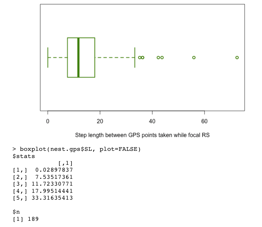
In the end, I settled on a simple rule: I compiled all of the step lengths between half-hour GPS points that were collected while the focal orangutan was resting in a day nest - i.e. when I knew the focal orangutan was not moving and so any movement in the track was error - and I used the “highest datum still within 1.5 IQR of the upper quartile” of the distribution of these step lengths. Simply put, I made a boxplot of the step lengths that I knew were ‘error steps,’ and I used the value of the upper whisker as the stopER value. I work with movement data from two different orangutan research sites and this method worked well, applied to each site individually. The sites have very different topography and canopy density, and I already knew from looking at the tracks and playing around with my function that I needed a much smaller stopER value for other (flatter, less dense canopy) site. By applying the ‘upper whisker of known error steps’ rule to each site, I found I was able to acheive a good error smoothing balance in the tracks from each site. I wonder if some version of this - getting a stopER value from the step lengths of known ‘error steps’ - could potentially be a promissing method for chosing the smoothing parameter value accross sites/species.
Massive Jumps
This second function deals with Problem 2, massive jumps. It takes 4 arguments:
- df - the data frame in which the data are stored
- X and Y - the names or numeric indices of the columns in df where the X and Y coordinates are stored
- maxJump - the maximum step length that would make ecological sense - i.e. anything more than this will get smoothed out
Like the other function, this function returns two new columns, called Xadj and Yadj, with adjusted points (and the same point coordinates as before where no adjustment was applied).
average_massive_jumps <- function(df, X, Y, maxJump) {
  if (nrow(df) > 1) {

    # START ---------- bringing in outlying starting points
    if (sqrt( ((df[1, X] - df[2, X])^2) + ((df[1, Y] - df[2, Y])^2) ) > maxJump ) {
      df[1, X] <- df[2, X]
      df[1, Y] <- df[2, Y]
    }

    # END ---------- bringing in outlying ending points
    if (sqrt( ((df[nrow(df), X] - df[(nrow(df)-1), X])^2) + ((df[nrow(df), Y] - df[(nrow(df)-1), Y])^2) ) > maxJump ) {
      df[nrow(df), X] <- df[(nrow(df)-1), X]
      df[nrow(df), Y] <- df[(nrow(df)-1), Y]
    }
  }

    # MIDDLE ---------- averaging midway outliers back in
  if (nrow(df)>2) {
    for (i in 2:(nrow(df)-1)) {
      if ( (sqrt( ((df[i, X] - df[i+1, X])^2) + ((df[i, Y] - df[i+1, Y])^2) ) > maxJump) &&
           (sqrt( ((df[i+1, X] - df[i+2, X])^2) + ((df[i+1, Y] - df[i+2, Y])^2) ) > maxJump) ) {
        df[i+1, X] <- mean(c(df[i, X], df[i+2, X]))
        df[i+1, Y] <- mean(c(df[i, Y], df[i+2, Y]))
      }
    }
  }
  return(df[, c(X,Y)])
}
So this function also does basically 3 things: 1) Reaches out from the first point to the next and if this step length is more than the maxJump distance, it pulls that first point in to where the second point is. 2) Reaches back from the last point to the previous, and if this step length is more than the maxJump distance, it pulls that last point in to where the second-last point is. 3) Loops through all of the points in the track, and checks the next two step lengths - if both of the next two steps are longer than the maxJump length, then it pulls the next point (i.e. the point in the middle of the two super long steps) back in line and puts it in between the point before it (the current point) and the point after it. Another way of saying this is that it looks for big spikes (that jump farther than the maxJump value) and it pulls the spikey point back in line with the points before and after it.
I found choosing the maxJump value to be a lot easier and less of a balancing act that the stopER value for the other function. I just made a histogram of all of the step lengths in my entire dataset and there were some very clear outliers. I manually checked (looked at the track, checked the behavioural data) many of the outliers, as well as several of the higher values that were in the tail of the distribution. In the end, for this site, I settled on a cut off of 600 meters. Of course, this could miss some error-made massive jumps that were shorter than 600 meters, but I didn’t want to risk smoothing out some big steps that were actually caused my unhabituated orangutans moving very fast. 1
Implementation station
There is no grouping done within the functions, so they needs to be wrapped in a loop or an apply function if they are to be applied to multiple non-consecutive/independent tracks. It’s also vital to make sure that your data are already sorted and so the rows in your dataframe are in the correct temporal order in which the locations occurred.
The implementation is a little clunky, but it gets the job done…
#initialize the output columns in my main dataframe
gps$Xadj <- NA
gps$Yadj <- NA

#run a loop that works with one follow at a time
for (i in 1:length(unique(gps$FolNum))) {

  #subset the data to get just this follow
  sub <- droplevels(subset(gps, gps$FolNum == unique(gps$FolNum)[i]))

  ## AVERAGING OUT MESSY STOPS
  sub[, c("Xadj", "Yadj")] <- average_messy_stops(sub, "X", "Y", 18)

  ## AVERAGING OUT MASSIVE JUMPS
  sub[, c("Xadj", "Yadj")] <- average_massive_jumps(sub, "Xadj", "Yadj", 600)

  #insert these new values into the right rows on the main dataframe
  gps[(match(sub$DateTime, gps$DateTime)), c("Xadj", "Yadj")] <- sub[, c("Xadj", "Yadj")]

  rm(sub)
}
rm(i)

#check out the data again
str(gps)
## 'data.frame':    68 obs. of  8 variables:
##  $ FolNum  : int  19 19 19 19 19 19 19 19 19 19 ...
##  $ Focal   : Factor w/ 2 levels "Pi","Roger": 2 2 2 2 2 2 2 2 2 2 ...
##  $ PtType  : Factor w/ 5 levels "FIND","LOST",..: 3 5 5 5 5 5 5 5 5 5 ...
##  $ DateTime: POSIXct, format: "2014-07-13 05:57:00" "2014-07-13 06:00:00" ...
##  $ X       : num  474432 474428 474449 474440 474422 ...
##  $ Y       : num  172843 172832 172827 172823 172831 ...
##  $ Xadj    : num  474430 474430 474445 474445 474428 ...
##  $ Yadj    : num  172837 172837 172825 172825 172830 ...
summary(gps)
##      FolNum      Focal          PtType      DateTime
##  Min.   : 19   Pi   :40   FIND     : 1   Min.   :2014-07-13 05:57:00
##  1st Qu.: 19   Roger:28   LOST     : 1   1st Qu.:2014-07-13 13:52:30
##  Median : 82              MORNNEST : 2   Median :2015-10-03 13:15:00
##  Mean   : 63              NIGHTNEST: 2   Mean   :2015-04-14 23:19:01
##  3rd Qu.:102              RANGE    :62   3rd Qu.:2015-11-09 08:07:30
##  Max.   :102                             Max.   :2015-11-09 16:07:00
##        X                Y               Xadj             Yadj
##  Min.   :474418   Min.   :172600   Min.   :474428   Min.   :172825
##  1st Qu.:474429   1st Qu.:172831   1st Qu.:474428   1st Qu.:172830
##  Median :474496   Median :173203   Median :474498   Median :173207
##  Mean   :474551   Mean   :173335   Mean   :474551   Mean   :173344
##  3rd Qu.:474604   3rd Qu.:173977   3rd Qu.:474606   3rd Qu.:173977
##  Max.   :474873   Max.   :174284   Max.   :474873   Max.   :174284
Now, let’s plot it and see the difference…

Figure 1: The original X and Y coordinates
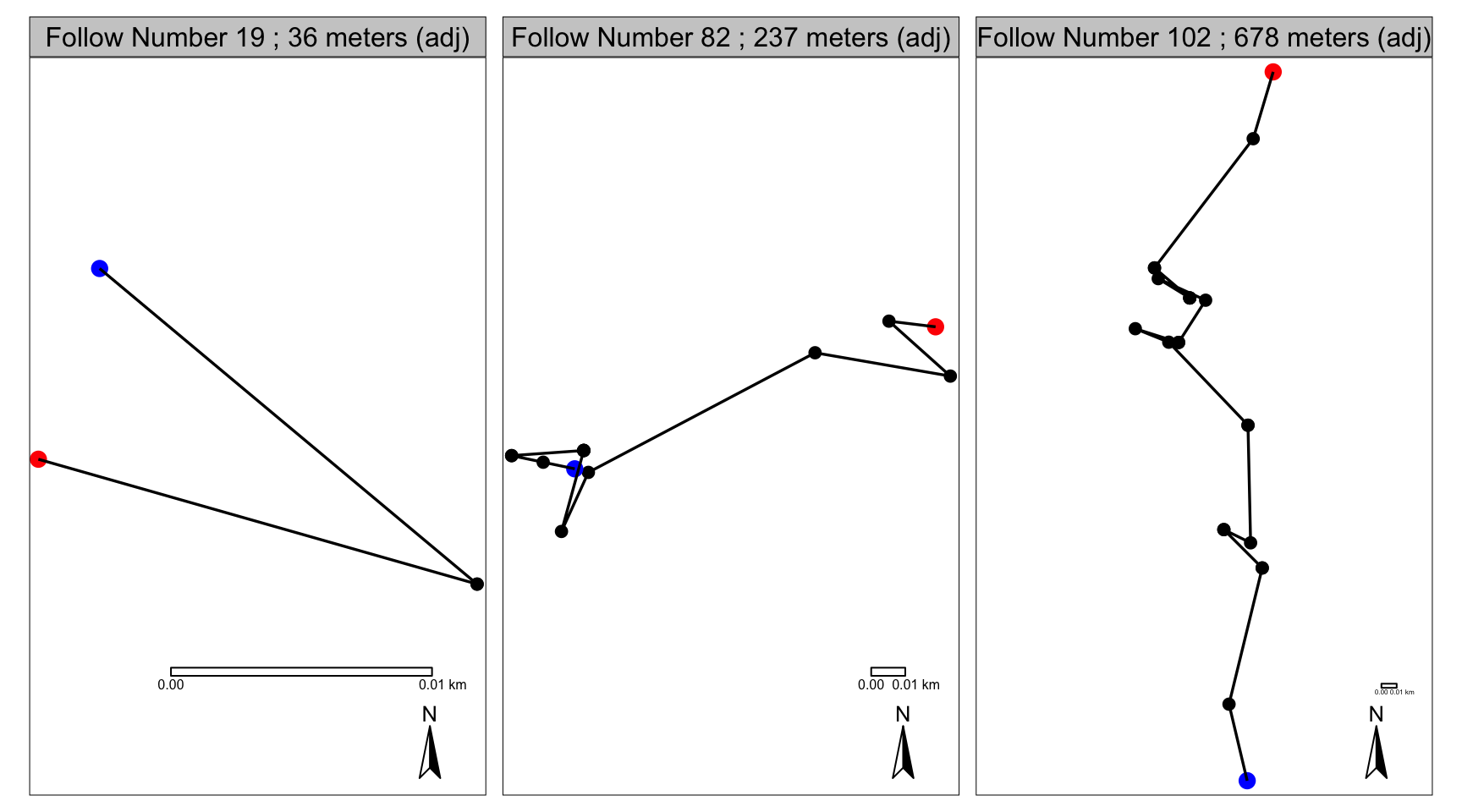
Figure 2: The adjusted X and Y coordinates
Et voilà! Now we have smoother tracks with more accurate DJLs! Of course, they’re not perfect, but I’m definitely happier with these tracks and these measurements that I was with the originals. Roger in his single tree in follow number 19 now makes a lot more sense. He probably did actually travel about 36 meters that day - back and forth across that huge tree’s crown. Pi in follow number 82 no longer has that impossible mad dash south and back north, and a lot of the noise is also now gone from around the start and end of her follow. Not as much has changed for Pi in follow number 102, except for some noise is gone from around stopping points, so her DJL has decreased a little bit.
Parting thoughts
I think one of the big draw backs to this method is that in some ways it seems really arbitrary - picking the stopER and the maxJump values. The chosen values really need to walk that line between under and over-smoothing, and I would imagine that without an intimate knowledge of the study species and the data collection protocols, and maybe without having actually followed a moving animal while watching the gps track jump around on the screen, it would be harder to pick appropriate values for these parameters. If using collar data, I suppose it could be possible to do behavioral observation that seek to validate/correlate behaviours with not only certain movement patterns, but also certain error patterns, which would then allow for appropriate estimation of these parameters. I’m really keen to know how others have approached and dealt with problems of GPS error. I can imagine using browning bridges movement modelling, or even kernel smoothing of some kind, to model a ‘highest probability path’ or something like that, but honestly, for my purposes that really seemed like overkill…. If you know of anything like this though, or any other way that this problem has been approached/solved, please let me know! :)
Of course, adding an angle component to this function could help with this, i.e. only adjust points if the enclosed angle of two steps longer than
maxJumpis less than a certain value. This would prevent any adjustments from being applied if there are simply two long steps, one after the other moving in a directional manner. If there was an angle component, then themaxJumpvalue could be smaller without risking so much over-smoothing - assuming you don’t expect your animal to do any very long back-and-forths… So, yes, lots of improvements could be made to these functions! A lot will depend on the study system and the way the data is collected too, but for what I was doing, this worked fine.↩