Maps on maps on maps
I recently figured out how to do something that I’ve been trying to do for a while: Plot geom_sf objects (spatial points, lines, polygons, etc) onto ggmaps (i.e. basically a google map background), in such a way that everything easily lines up properly. I won’t get into the nitty gritty and ins and outs of all of the components here, or else we’ll be here all day. Instead, I’ll just quickly go through an example and show what worked for me. I spent a lot of time reading through other blogs, stackoverflow answers, etc. and tried a million different things, and finally found a simple solution that actually worked. So, just in case you are having the same problem, maybe the same solution will also work for you! I’ll go through the whole sh’bang, building a map from scratch, but if you’re not interested in this, you can just skip ahead to the most important parts.
The components
Ok, let’s say that I have 4 components that I want to get all on the same plot:
- A background map of the terrain,
- A home range calculated using adehabitatHR package (ie.e a
SpatialPologonobject), - Some GPS waypoints, also in .gpx format,
- A track in .gpx format that I want as a polygon shape.
For our purposes today, I’ll just use some random bits and pieces of fake data and throw them all together on a map of Borneo.
First, we load the packages we need.
library(ggmap) #to get the background maps; note: THIS ALSO LOADS ggplot2
library(sf) #for plotting spatial objects with ggplot2
library(ggspatial) #for adding mappy things (scale, North arrow) to our plots
library(adehabitatHR) #for calculating a home range
library(rgdal) #for bringing in .GPX files
library(viridis) #for nice color scales for plotting
Background terrain map
For the background terrain map, I will use the ggmap package by David Kahle. To get background maps with this package, you need to get a Google Maps API - you can register for an API here - choose ‘Maps’. You need to provide a credit card, but you can get a lot of maps for free (I think it told me I get a 300 CHF credit in my first year for free), and after that the prices are very reasonable (more pricing info here, and also see what Kahle has posted about it here). After you register, you’ll get a unique key (just a long string of numbers and letters) that you need to use in order to get any maps (keep your key private!).
First, put in your Google API…
register_google(key = xxx) #put your API where the xxx isUse the get_map function…
#example - all of Borneo
borneo <- get_map(location = c(lon = 114, lat = 1.3),  #coordiantes of the middle of the map
              zoom = 6, #higher numbers = closer zoom in
              maptype = "terrain", #there are many different options, see ?get_map for details
              color = "color") #color or bw for greyscale
#> Source : https://maps.googleapis.com/maps/api/staticmap?center=1.3,114&zoom=6&size=640x640&scale=2&maptype=terrain&language=en-EN&key=xxx
ggmap(borneo)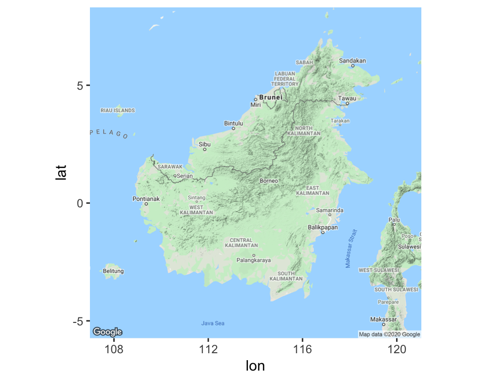
#now zoom in on our area of interest
EastKutai_zoom <- get_map(location = c(lon = 116.755, lat = 1.567), #coordiantes of the middle of the map
zoom = 12, #higher numbers = closer zoom in
maptype = "terrain", #there are many different options, see ?get_map for details
color = "color") #color or bw for greyscale
#> Source : https://maps.googleapis.com/maps/api/staticmap?center=1.567,116.755&zoom=12&size=640x640&scale=2&maptype=terrain&language=en-EN&key=xxx
ggmap(EastKutai_zoom)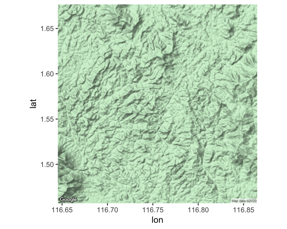 Boom! It’s a map! Good start.
You can check out this pdf for a helpful overview of the different types of background maps that you can get using the get_map function, as well as some other helpful info about the ggmap package.
A SpatialPolygonDataFrame object
So, if you’ve calculated a home range or whatnot using adehabitatHR or any other sp-based package, then you’ll have some sort of sp object, which needs to be converted to an sf object before it can be added as a geom_sf layer.
So, for this example, I’ve loaded a home ranges calculated using the kernelUD function in adehabitatHR and then converted to a SpatialPolygonsDataFrame using the getverticesHR function.
str(homerange) #take a look at the object
#> Formal class 'SpatialPolygonsDataFrame' [package "sp"] with 5 slots
#>   ..@ data       :'data.frame':  1 obs. of  2 variables:
#>   .. ..$ id  : Factor w/ 1 level "homerange": 1
#>   .. ..$ area: num 288
#>   ..@ polygons   :List of 1
#>   .. ..$ :Formal class 'Polygons' [package "sp"] with 5 slots
#>   .. .. .. ..@ Polygons :List of 1
#>   .. .. .. .. ..$ :Formal class 'Polygon' [package "sp"] with 5 slots
#>   .. .. .. .. .. .. ..@ labpt  : num [1:2] 474193 173617
#>   .. .. .. .. .. .. ..@ area   : num 2878419
#>   .. .. .. .. .. .. ..@ hole   : logi FALSE
#>   .. .. .. .. .. .. ..@ ringDir: int 1
#>   .. .. .. .. .. .. ..@ coords : num [1:370, 1:2] 472939 472932 472925 472923 472927 ...
#>   .. .. .. ..@ plotOrder: int 1
#>   .. .. .. ..@ labpt    : num [1:2] 474193 173617
#>   .. .. .. ..@ ID       : chr "homerange"
#>   .. .. .. ..@ area     : num 2878419
#>   ..@ plotOrder  : int 1
#>   ..@ bbox       : num [1:2, 1:2] 472923 172301 475336 174935
#>   .. ..- attr(*, "dimnames")=List of 2
#>   .. .. ..$ : chr [1:2] "x" "y"
#>   .. .. ..$ : chr [1:2] "min" "max"
#>   ..@ proj4string:Formal class 'CRS' [package "sp"] with 1 slot
#>   .. .. ..@ projargs: chr "+proj=utm +zone=50 +ellps=WGS84"

#convert it to an sf object
homerange_sf <- st_as_sf(homerange)

#take a look at it
ggplot() +
  geom_sf(data = homerange_sf)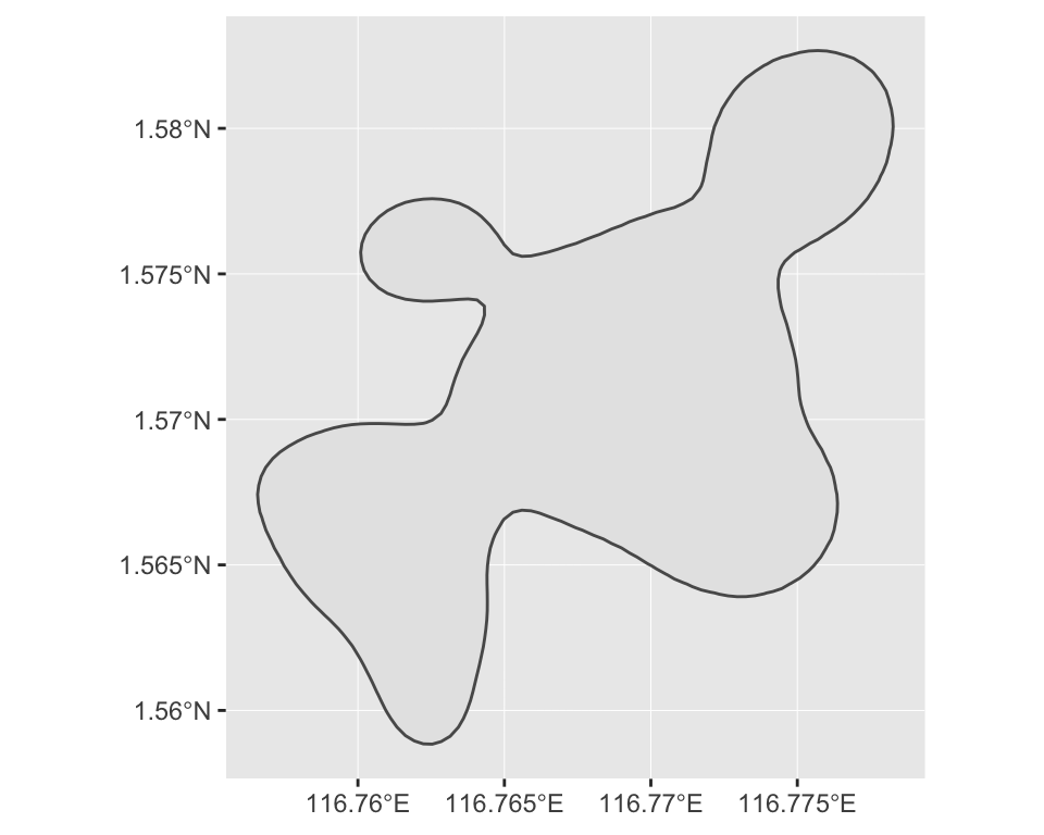
Tracks and points from .GPX files
If you’ve collected data on a handheld GPS unit, you may have experience working with .GPX files - tracks and waypoints can all be stored as .GPX file type. The following code imports waypoints from a .GPX files and converts them into a “POINT” sf object.
#check out the layers of the GPX file
layers <- ogrListLayers(point_GPX_filepath)

layers
#> [1] "waypoints"    "routes"       "tracks"       "route_points"
#> [5] "track_points"
#> attr(,"driver")
#> [1] "GPX"
#> attr(,"nlayers")
#> [1] 5

#read in the correct layer (in this case waypoints which is layer 1)
landmarks <- readOGR(point_GPX_filepath,
                  layer=layers[1])
#> OGR data source with driver: GPX
#> Source: "/Users/amashbury/Google Drive/Only REY/Alie's Data Space/static/posts/2019-10-04-maps-on-maps-on-maps_files/points.GPX", layer: "waypoints"
#> with 3 features
#> It has 26 fields

#set the spatial projection
landmarks <- spTransform(landmarks, CRSobj = "+proj=utm +zone=50 +north +ellps=WGS84")

#convert it to an sf object
landmarks_sf <- st_as_sf(landmarks[c("time", "name")])


#take a look at it
ggplot() +
  geom_sf(data = landmarks_sf)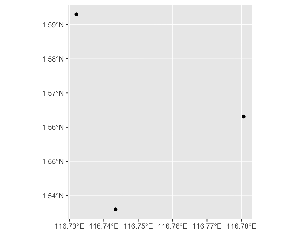
And here, the following code imports the track(s) from a .GPX files and converts it into a “LINESTRING” sf object. Then, because this track is meant to represent borders of an area which I’d rather have represented as a polygon, I’ll convert it to an “POLYGON” sf object.
#check out the layers of the GPX file
layers <- ogrListLayers(track_GPX_filepath)

layers
#> [1] "waypoints"    "routes"       "tracks"       "route_points"
#> [5] "track_points"
#> attr(,"driver")
#> [1] "GPX"
#> attr(,"nlayers")
#> [1] 5

#read in the correct layer (in this case track which is layer 3)
border_track <- readOGR(track_GPX_filepath,
                  layer=layers[3])
#> OGR data source with driver: GPX
#> Source: "/Users/amashbury/Google Drive/Only REY/Alie's Data Space/static/posts/2019-10-04-maps-on-maps-on-maps_files/track.GPX", layer: "tracks"
#> with 1 features
#> It has 13 fields

#set the spatial projection
border_track <- spTransform(border_track, CRSobj = "+proj=utm +zone=50 +north +ellps=WGS84")

#convert it to an sf object
border_track_sf <- st_as_sf(border_track["name"])

#take a look at it
ggplot() +
  geom_sf(data = border_track_sf)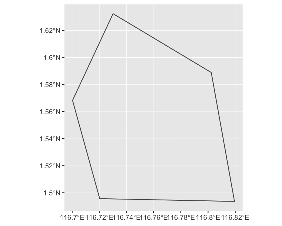
#convert line to polygon
border_poly_sf <- st_cast(border_track_sf, "POLYGON")

#take a look at it
ggplot() +
  geom_sf(data = border_poly_sf)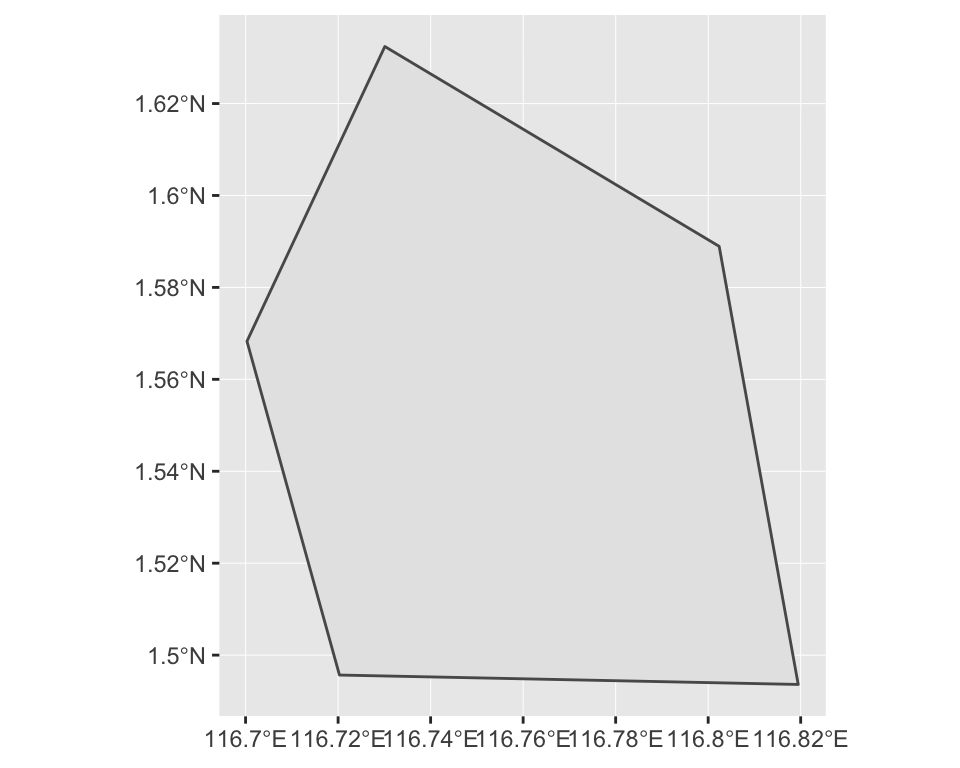
Put it all together
And now, I’ll stack it all together into one single map…
#start with the ggmap function, and give it your chosen map
ggmap(EastKutai_zoom) +
  # then add in each of the sf objects...

  #add the border first, and shade the inside of the polygone
  geom_sf(data = border_poly_sf,
          mapping = aes(linetype = name),
          alpha = 0.5,
          fill = "white",
          color = "black",
          show.legend = "line",
          size = 1.2,
          inherit.aes = FALSE) +
  scale_linetype_manual("", values = "dashed",
                        labels = "Border",
                        guide = guide_legend(override.aes = list(linetype = "dashed",
                                                                 fill = NA,
                                                                 shape = NA,
                                                                 alpha = 0,
                                                                 color = "black",
                                                                 size = 0.8))) +
  #now add the home range on top of this...
  geom_sf(data = homerange_sf,
          mapping = aes(fill = id),
          alpha = 0.8,
          color = "grey30",
          show.legend = "poly",
          inherit.aes = FALSE) +
    scale_fill_manual("", values = viridis(3)[3],
                    labels = "Oma's homerange",
                    guide = guide_legend(override.aes = list(linetype = "solid",
                                                             fill = viridis(3)[3],
                                                             shape = NA,
                                                             alpha = 1,
                                                             color = "grey30"))) +
  #and then add the landmark points on top
  geom_sf(data = landmarks_sf,
          mapping = aes(color = name,
                        shape = name),
          size = 3,
          show.legend = "point",
          inherit.aes = FALSE) +
  scale_color_manual("",
                     values = plasma(4)[1:3],
                     guide = guide_legend(override.aes = list(linetype = "blank",
                                                              fill = NA))) +
  scale_shape_manual("",
                     values = 15:17,
                     guide = guide_legend(override.aes = list(linetype = "blank"))) +

  #set the CRS for the entire map
  coord_sf(crs = st_crs(4326)) +
  #now add some mappy things
  annotation_scale(location = "bl", width_hint = 0.4,
                   pad_x = unit(0.1, "in"),
                   pad_y = unit(0.2, "in"),
                   bar_cols = c("black", "white"),
                   line_col = "black",
                   text_col = "black") +
  annotation_north_arrow(location = "tl", which_north = "true",
                         pad_x = unit(0.3, "in"), pad_y = unit(0.3, "in"),
                         height = unit(0.5, "in"), width= unit(0.3, "in"),
                         style = north_arrow_orienteering(fill = c("black", "black"),
                                                          line_col = "black",
                                                          text_col = "black")) +
  #and some stylistic details
  theme_bw() +
  theme(axis.title.x = element_blank(),
        axis.title.y = element_blank())
#> Coordinate system already present. Adding new coordinate system, which will replace the existing one.
#> Warning in guide_merge.legend(init, x[[i]]): Duplicated override.aes is
#> ignored.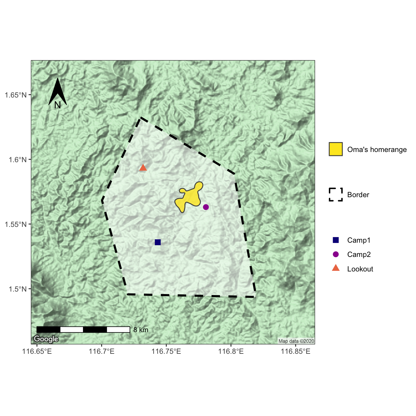
The most important parts
So, basically, the little things that made this (plotting a bunch of geom_sf layers onto a ggmap background) work for me, and that solved all of the weird errors and alighnment/projection problems I’d been having are the follow key points:
- Be explicit and include
data =andmapping =in eachgeom_sflayer. - Also include
inherit.aes = FALSEin eachgeom_sflayer. - Include
+ coord_sf(crs = st_crs(4326))in order to standardize the CRS accross all layers (Note: Include this even if the sf objects already have the same CRS!). You can also add other arguments in thecoord_sf()function, such asxlim = c(min, max)andylim = c(min, max)to crop the whole map, etc.
And that’s basically it! It’s actually all very simple, in hindsight (as difficult things usually are, I suppose). Happy mapping!
