
It's all fun(ctions) and games
When you’ve written the same code 3 times, write a function
— David Robinson (@drob) November 9, 2017
When you’ve given the same in-person advice 3 times, write a blog post
Fun fact: This tweet is actually what inspired me to start this website.
Secondly, he’s right, and we should definitely all be writing functions for bits and pieces of code that we are using over and over again. It keeps code clean, clear, and compartmentalized. It may be a bit confusing at first, but it pays off once you figure it out, I promise.
So, let’s write some functions!
The basics
To write a function, you use the function() function. When you run the function-making code, your new function will then become a part of your R Environment. If you’re using R Studio, you’ll see it pop up in the “Global Environment” pane (under the “Environment” tab in the top right (if you are using the default) position of the R Studio window). Once you’ve got the function in your R session Environment, then you can use it!
The diagram below gives a schematic drawing of what the overall syntax of a function looks like…
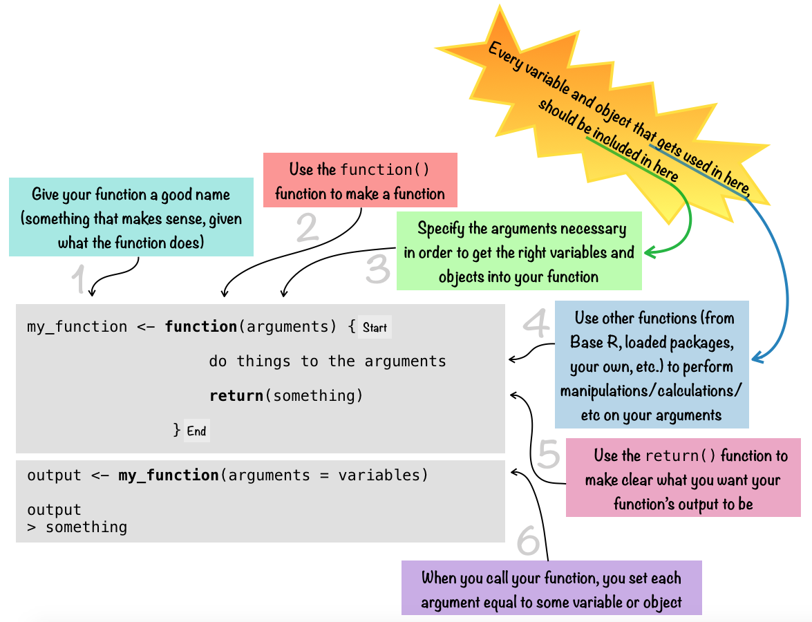
Note that the return() part of the function can be omitted, in which case your function will automatically output whatever the last thing is that was calcuated. For more simple functions especially, using return() is often overkill. But for more complicated functions that do a lot of computing, it can be really helpful to make explicit what will be outputted.
The following functions all take a single argument (pounds), and they compute the same output: pounds X 0.45359237; in other words, they convert pounds to kilograms. Notice all of the different options, and especially how the return() function works…
pounds_to_kilos_full <- function(pounds) {
  y <- pounds * 0.45359237
  return(y)
}

# which is also the same as...
pounds_to_kilos_med <- function(pounds) {
  return(pounds * 0.45359237)
}

# which is also the same as...
pounds_to_kilos_light <- function(pounds) {
  pounds * 0.45359237
}

# which is also the same as...
pounds_to_kilos_confusing1 <- function(pounds) {
  pounds * 10           #this computation will get done, but there won't be any output from it
  return(pounds * 0.45359237)    #this is in the return function, so it will be the output
}

# which is also the same as...
pounds_to_kilos_confusing2 <- function(pounds) {
  pounds * 10          #this computation will get done, but there won't be any output from it
  pounds * 0.45359237           #this is the last thing calculated, so it will be the output
}

# which is also the same as...
pounds_to_kilos_confusing3 <- function(pounds) {
  return(pounds * 0.45359237)   #this is in the return function, so it will be the output
  pounds * 10          #this computation will get done, but there won't be any output from it
}

# all 6 are the same...
pounds_to_kilos_full(pounds = 3)
#> [1] 1.360777
pounds_to_kilos_med(pounds = 3)
#> [1] 1.360777
pounds_to_kilos_light(pounds = 3)
#> [1] 1.360777
pounds_to_kilos_confusing1(pounds = 3)
#> [1] 1.360777
pounds_to_kilos_confusing2(pounds = 3)
#> [1] 1.360777
pounds_to_kilos_confusing3(pounds = 3)
#> [1] 1.360777
So regardless of what else goes on in the function, the value given in the return function is what is spit out. If there is no internal return function, the the last value computed is returned. One really important thing to notice is in the first function (pounds_to_kilos_full) at the top: inside this function, an object y is created. However, if you run this function in your R workspace, you will notice that this object does not appear in your R session “Environment.” This is one of the nice things about using functions - if you have intermediate steps in your processes that create objects which you don’t actually really need (except to get to the next step), those objects will exist only within the functions, and not clutter up your workspace.
Consider the next example in which I perform the same calculations outside and then inside a function…
#Side Note: let's just clear out this workspace before we continue
rm(list = ls(all.names = TRUE))

#do the computations without combining them into a function
y <- mean(1:10)
z <- y + 5
a <- z * 3
output <- a
output #look at the output
#> [1] 31.5

#show everything in the workspace
ls(all.names = TRUE)
#> [1] "a"      "output" "y"      "z"

#now, clear the workspace again
rm(list = ls(all.names = TRUE))

#make the function
boom <- function(x) {
  y <- mean(x)
  z <- y + 5
  a <- z * 3
  return(a)
}
#run it
output <- boom(x = 1:10)
output #look at the output
#> [1] 31.5

#show everything in the workspace
ls(all.names = TRUE)
#> [1] "boom"   "output"
So, you can see how, if you just run the calculations straight up, all of those objects y, z, a, output end up in your Environment. But, if you embed the calculations into a function, and run the function, then you only end up with boom (the function), and output (the final, return() object, the object that you wanted all along) in your Environment, which is much cleaner. Now imagine that the function does something more complex, and creates more objects along the way, and you want to run the function multiple times… then this discrepancy in “cleanliness” will really make a difference, and it would be much nicer to use a function.
Some examples
The following are some examples of relatively simple functions that I’ve written, that I find pretty handy…
Distance caluclation:
The following function is meant for situations wherin I want to calculate the step lengths (distances) between each point and the next point in a time series of locaitons. The function takes (as input) two vectors, meant to be the X and Y values of projected coordinates (imagine each as a column in a dataframe wherein each row is a location point), and calculates the distance between each one. To do this, it uses the standard distance formula \(d = \sqrt {\left( {x_1 - x_2 } \right)^2 + \left( {y_1 - y_2 } \right)^2 }\), and applies it along the vectors of X and Y coordinates (input as the X and Y arguments), first measuring between the first and second elements (X[1] and Y[1] to X[2] and Y[2]), then between the second and third (X[2] and Y[2] to X[3] and Y[3]), and so on, until it does so between the second last and the last (X[length(X)-1] and Y[length(Y)-1] to X[length(X)] and Y[length(X)]). The output is a vector of step lengths from each point to the next one, with the first position of the vector filled by an NA so that the output can be directly added to the dataframe, as a new column, and the first row of the dataframe (for which there is no step length because there is no preceeding location from which to measure) will have a step length of NA.
# generate some fake data, just X and Y coordinates
fake_data <- data.frame(cbind(Xcoord = sample(1:50, 10, replace = TRUE),
                              Ycoord = sample(1:50, 10, replace = TRUE)))
fake_data
#>    Xcoord Ycoord
#> 1      11      7
#> 2      25     21
#> 3      19     29
#> 4      17     44
#> 5      10     16
#> 6       5     37
#> 7      44     18
#> 8      20     40
#> 9      23     48
#> 10      8     27

# the function
measure_step_lengths <- function(X, Y) {
  SLs <- sqrt(
               ( ( X[1:(length(X)-1)] -
                        X[2:length(X)])^2) +
               ( (Y[1:(length(Y)-1)] -
                        Y[2:length(Y)])^2)
            )
  return(c(NA, SLs))
}


# run it to see output
measure_step_lengths(X = fake_data$Xcoord, Y = fake_data$Ycoord)
#>  [1]        NA 19.798990 10.000000 15.132746 28.861739 21.587033 43.382024
#>  [8] 32.557641  8.544004 25.806976

# this time run it, but append step lengths to the dataframe
fake_data$SL <- measure_step_lengths(X = fake_data$Xcoord, Y = fake_data$Ycoord)

#now take a look at the data
fake_data
#>    Xcoord Ycoord        SL
#> 1      11      7        NA
#> 2      25     21 19.798990
#> 3      19     29 10.000000
#> 4      17     44 15.132746
#> 5      10     16 28.861739
#> 6       5     37 21.587033
#> 7      44     18 43.382024
#> 8      20     40 32.557641
#> 9      23     48  8.544004
#> 10      8     27 25.806976
Get unique names from messy columns: The following function is one I used a lot while cleaning up orangutan party member data for summary analyses. I used this function on two different tables: a follow overview table - one row per focal day; and an activity table - one row for every 2-minute instantaenous sample. Both tables have columns in which the party members (other orangutans who were in association with the focal during that day / at that 2-minute interval) are listed in wide format - so one party member id per cell, in side-by-side columns. These data are not always clean, sometimes they get coded in as factors and sometimes character strings, with variations in capitalization and different individuals in different rows on different days / at different times. Often, I want to know all of the different party members for a particular subset of the data (for example, all follows of a certain focal individual). So, this function just takes two arguments, the name of the dataframe, and the indices or names of the party member columns, cleans them up a bit, and outputs all unique entries.
#generate some fake data with messy party columns
fake_data <- data.frame(cbind(FollowNumber = 1:10,
                              Focal = rep("PI", 10),
                              PM1 = c(NA, "THEO", "theo", "TOB", NA, "BELLA", "Bella", "TOB", "Roger", "Ripley"),
                              PM2 = c(NA, "tob", "ROGER", "Theo", NA, "Ripley", NA, NA, NA, NA),
                              PM3 = c(NA, NA, NA, "ROger", NA, NA, "RIPLEY", NA, NA, NA)))

fake_data #take a look at it
#>    FollowNumber Focal    PM1    PM2    PM3
#> 1             1    PI   <NA>   <NA>   <NA>
#> 2             2    PI   THEO    tob   <NA>
#> 3             3    PI   theo  ROGER   <NA>
#> 4             4    PI    TOB   Theo  ROger
#> 5             5    PI   <NA>   <NA>   <NA>
#> 6             6    PI  BELLA Ripley   <NA>
#> 7             7    PI  Bella   <NA> RIPLEY
#> 8             8    PI    TOB   <NA>   <NA>
#> 9             9    PI  Roger   <NA>   <NA>
#> 10           10    PI Ripley   <NA>   <NA>


# give the party columns and it outputs a vector of all unique party IDs
get_all_unique_party_members <- function(df, party_id_cols) {

  # convert all ids to character strings (in case they are factors)
  df[,party_id_cols] <- lapply(df[,party_id_cols], as.character)

  # convert all ids to upper case, to standardize casing
  df[,party_id_cols] <- lapply(df[,party_id_cols], toupper)

  # stack all the columns into one long vector of names
  all_ids <- unname(unlist(df[,party_id_cols]))

  # keep only one instance of each name (i.e. unique ids)
  unique_ids <- unique(na.omit(all_ids))

  # return those unique ids
  return(unique_ids)
}

# use the function to get a vector of all unique party members in the dataframe
get_all_unique_party_members(df = fake_data, party_id_cols = 3:5)
#> [1] "THEO"   "TOB"    "BELLA"  "ROGER"  "RIPLEY"

# you can also use the party column names
get_all_unique_party_members(df = fake_data, party_id_cols = c("PM1", "PM2", "PM3"))
#> [1] "THEO"   "TOB"    "BELLA"  "ROGER"  "RIPLEY"
Note that, if you put the arguments into the function in the order that the function expects them - in the above case, this is df and then party_id_cols - then it’s not necessary to have df = __ and party_id_cols = __. It would work the same to just run get_all_unique_party_members(fake_data, 3:5). However, it’s good practice to name your arguments and is especially important incase you put them in in a weird order, or if there are optional arguments (not covered in this post). I also once lost a whole day ripping my hair out trying to debug a function that had worked perfectly the day before - it ended up that I was just calling the arguments (unnamed!) in the wrong order… so… learn from my mistakes. Name your arguments when you call your functions.
Another handy function that I wrote can be seen in my past post about colour palettes, about a quarter of the way down the post (the seepalette function). Two rather more complex examples (probably more complex than they should be) can be found in my past post about minimizing GPS error in animal tracks.
A few notes
Remember that any object that is needed inside the function should be passed to it as an argument. A common error that I see when people are writing their first functions is something like this…
x <- 5

add_up <- function(y) {
  return(y + x)
}

add_up(y = 2)
#> [1] 7
So you can see how the object x is created in the Global Environment, but then it’s used in the function. If x is a constant and will always be the same (i.e. in this example, x will ALWAYS be 5, and you just want your function to always y + 5), then it’s better to just use that constant in the function, rather than an object whose value needs to be assigned beforehand. But if x is subject to change values, and if x is required for the function to work, then x should be included as an argument within the function itself - ie. add_up <- function(x, y) and then you pass x into the function by setting x = whatever when you call the function. Otherwise you’re just setting yourself up for a lot of debugging work (ok, maybe not with such a simple function as this, but definitely with something more complex).
You can also set default values for arguments, when you define the function. In other words, within the function() defining function itself, set an argument = to something. This way, if you don’t set that argument when you call the function, it will use the ‘default’ value instead.
# set the x argument default to 5
add_up <- function(y, x = 5) {
  return(y + x)
}

add_up(y = 2) # in this case, x defaults to 5
#> [1] 7
add_up(y = 2, x = 10) # in this case, the default x is overridden, and x is set to 10
#> [1] 12
Final thoughts
A final thing to keep in mind is that one function should complete one task. So even if you have 5 procedural steps that you want to do, it’s better to write five small functions, one for each step, than one big huge function that does all 5 things. I read somewhere once that ecologists (not sure why ecologists - if it’s just ecologists, or if the writer could only speak for ecologists, but anyways) tend to write functions that do too much. At the time, I was struggling to write a function that, indeed, did way too much, and just reading this helped me to realize I needed to break it down into smaller chunks of the process that I wanted done, and write a function for each chunk.
There is lots more that can be said about functions, but hopefully this is enough to get your started! Other potentially helpful links, including some that deal with more advanced concepts in function writing are:
- A nice introduction to writing functions, on a website aptly named Nice R Code.
- The official R documentation on writing your own function.
- The section on R functions in the official tidyverse style guide by Hadley Wickham.
- The section on writing R functions in Hadley Wickham’s Advanced R book.