
Flipping and flopping without floundering
Changing my data from wide to long format, or vice versa was somehow always a headache. Eventhough I did this a lot, it just DID NOT stick in my head for the longest time. Everytime, I had to google it, and then work through at least 5 failed attempts before I’d get it. Therefore, this totally warrants a blog post, ya?
I recently started using tidyr’s spread() and gather() functions to do this, and I find them a lot more intuitive than the alternatives (the tidyverse strikes again), so that’s what I’ll focus on here. Other options, would be the reshape2 package, but honestly, I haven’t found any clear advantages of it over tidyr’s version, so I’ll ignore it for now…
Set up for some flippity floppity
So, let’s start by making some data that is in wide format. Let’s imagine we have 10 focal orangutans. Each orangutan has been followed to night-nest many times. Night nests can be built in one of 4 positions. So, each orangutan has a count of the number of times it has built a nest in each position. We’ll make the data in wide format with one column for the orangutan names, one column for the orangutan age-sex class, and one column for each nest position, where the counts will be held…
library(tidyverse)
## Warning: package 'ggplot2' was built under R version 3.5.2
## Warning: package 'tibble' was built under R version 3.5.2
## Warning: package 'dplyr' was built under R version 3.5.2
## Warning: package 'stringr' was built under R version 3.5.2
set.seed(100)

#generate the 6 columns
data <- as_tibble(cbind(Individual = c("Pi", "Roger", "Luaqlas", "Englas", "Boy", "Mindy", "Milo", "Loki", "Monster", "Jip"),
                        ASclass = c("AdultFemale", "FlangedMale", "AdolescentFemale", "AdolescentMale", "AdolescentMale",
                                    "AdultFemale", "AdolescentFemale", "FlangedMale", "FlangedMale", "UnflangedMale"),
                        NestPos1 = sample(1:20, 10, replace = TRUE),
                        NestPos2 = sample(1:20, 10, replace = TRUE),
                        NestPos3 = sample(1:20, 10, replace = TRUE),
                        NestPos4 = sample(1:20, 10, replace = TRUE)))
#check it
str(data)
## Classes 'tbl_df', 'tbl' and 'data.frame':    10 obs. of  6 variables:
##  $ Individual: chr  "Pi" "Roger" "Luaqlas" "Englas" ...
##  $ ASclass   : chr  "AdultFemale" "FlangedMale" "AdolescentFemale" "AdolescentMale" ...
##  $ NestPos1  : chr  "7" "6" "12" "2" ...
##  $ NestPos2  : chr  "13" "18" "6" "8" ...
##  $ NestPos3  : chr  "11" "15" "11" "15" ...
##  $ NestPos4  : chr  "10" "19" "7" "20" ...

#fix the numeric columns
data[,3:6] <- lapply(data[,3:6], as.numeric)

#check it all
data
## # A tibble: 10 x 6
##    Individual ASclass          NestPos1 NestPos2 NestPos3 NestPos4
##    <chr>      <chr>               <dbl>    <dbl>    <dbl>    <dbl>
##  1 Pi         AdultFemale             7       13       11       10
##  2 Roger      FlangedMale             6       18       15       19
##  3 Luaqlas    AdolescentFemale       12        6       11        7
##  4 Englas     AdolescentMale          2        8       15       20
##  5 Boy        AdolescentMale         10       16        9       14
##  6 Mindy      AdultFemale            10       14        4       18
##  7 Milo       AdolescentFemale       17        5       16        4
##  8 Loki       FlangedMale             8        8       18       13
##  9 Monster    FlangedMale            11        8       11       20
## 10 Jip        UnflangedMale           4       14        6        3
summary(data)
##   Individual          ASclass             NestPos1        NestPos2
##  Length:10          Length:10          Min.   : 2.00   Min.   : 5.0
##  Class :character   Class :character   1st Qu.: 6.25   1st Qu.: 8.0
##  Mode  :character   Mode  :character   Median : 9.00   Median :10.5
##                                        Mean   : 8.70   Mean   :11.0
##                                        3rd Qu.:10.75   3rd Qu.:14.0
##                                        Max.   :17.00   Max.   :18.0
##     NestPos3       NestPos4
##  Min.   : 4.0   Min.   : 3.00
##  1st Qu.: 9.5   1st Qu.: 7.75
##  Median :11.0   Median :13.50
##  Mean   :11.6   Mean   :12.80
##  3rd Qu.:15.0   3rd Qu.:18.75
##  Max.   :18.0   Max.   :20.00
Gather and Flip
Ok, so now let’s say we want to FLIP the data down into LONG form - so we want one column for Individual, one column for ASclass, one column for NestPosition, and one column for the Counts of each nest position. As such, each Individual and ASclass pairing will be repeated FOUR times - once per nest position. The values in the NestPosition column should be 1, 2, 3, and 4, repeated for each Individual.
I will use the gather() function from the tidyr package…
#GATHER ((these two next lines of code are exactly the same))
data.long <- data %>% gather(NestPosition, Counts, 3:6) #use the column indices
data.long <- data %>% gather(NestPosition, Counts, c("NestPos1", "NestPos2", "NestPos3", "NestPos4")) #use the column names

#look at the whole thing
data.long %>% print(n = Inf)
## # A tibble: 40 x 4
##    Individual ASclass          NestPosition Counts
##    <chr>      <chr>            <chr>         <dbl>
##  1 Pi         AdultFemale      NestPos1          7
##  2 Roger      FlangedMale      NestPos1          6
##  3 Luaqlas    AdolescentFemale NestPos1         12
##  4 Englas     AdolescentMale   NestPos1          2
##  5 Boy        AdolescentMale   NestPos1         10
##  6 Mindy      AdultFemale      NestPos1         10
##  7 Milo       AdolescentFemale NestPos1         17
##  8 Loki       FlangedMale      NestPos1          8
##  9 Monster    FlangedMale      NestPos1         11
## 10 Jip        UnflangedMale    NestPos1          4
## 11 Pi         AdultFemale      NestPos2         13
## 12 Roger      FlangedMale      NestPos2         18
## 13 Luaqlas    AdolescentFemale NestPos2          6
## 14 Englas     AdolescentMale   NestPos2          8
## 15 Boy        AdolescentMale   NestPos2         16
## 16 Mindy      AdultFemale      NestPos2         14
## 17 Milo       AdolescentFemale NestPos2          5
## 18 Loki       FlangedMale      NestPos2          8
## 19 Monster    FlangedMale      NestPos2          8
## 20 Jip        UnflangedMale    NestPos2         14
## 21 Pi         AdultFemale      NestPos3         11
## 22 Roger      FlangedMale      NestPos3         15
## 23 Luaqlas    AdolescentFemale NestPos3         11
## 24 Englas     AdolescentMale   NestPos3         15
## 25 Boy        AdolescentMale   NestPos3          9
## 26 Mindy      AdultFemale      NestPos3          4
## 27 Milo       AdolescentFemale NestPos3         16
## 28 Loki       FlangedMale      NestPos3         18
## 29 Monster    FlangedMale      NestPos3         11
## 30 Jip        UnflangedMale    NestPos3          6
## 31 Pi         AdultFemale      NestPos4         10
## 32 Roger      FlangedMale      NestPos4         19
## 33 Luaqlas    AdolescentFemale NestPos4          7
## 34 Englas     AdolescentMale   NestPos4         20
## 35 Boy        AdolescentMale   NestPos4         14
## 36 Mindy      AdultFemale      NestPos4         18
## 37 Milo       AdolescentFemale NestPos4          4
## 38 Loki       FlangedMale      NestPos4         13
## 39 Monster    FlangedMale      NestPos4         20
## 40 Jip        UnflangedMale    NestPos4          3

str(data.long)
## Classes 'tbl_df', 'tbl' and 'data.frame':    40 obs. of  4 variables:
##  $ Individual  : chr  "Pi" "Roger" "Luaqlas" "Englas" ...
##  $ ASclass     : chr  "AdultFemale" "FlangedMale" "AdolescentFemale" "AdolescentMale" ...
##  $ NestPosition: chr  "NestPos1" "NestPos1" "NestPos1" "NestPos1" ...
##  $ Counts      : num  7 6 12 2 10 10 17 8 11 4 ...
summary(data.long)
##   Individual          ASclass          NestPosition           Counts
##  Length:40          Length:40          Length:40          Min.   : 2.00
##  Class :character   Class :character   Class :character   1st Qu.: 7.00
##  Mode  :character   Mode  :character   Mode  :character   Median :11.00
##                                                           Mean   :11.03
##                                                           3rd Qu.:15.00
##                                                           Max.   :20.00
It’s actually so simple that it surprises me every time. Let me try to break this down:
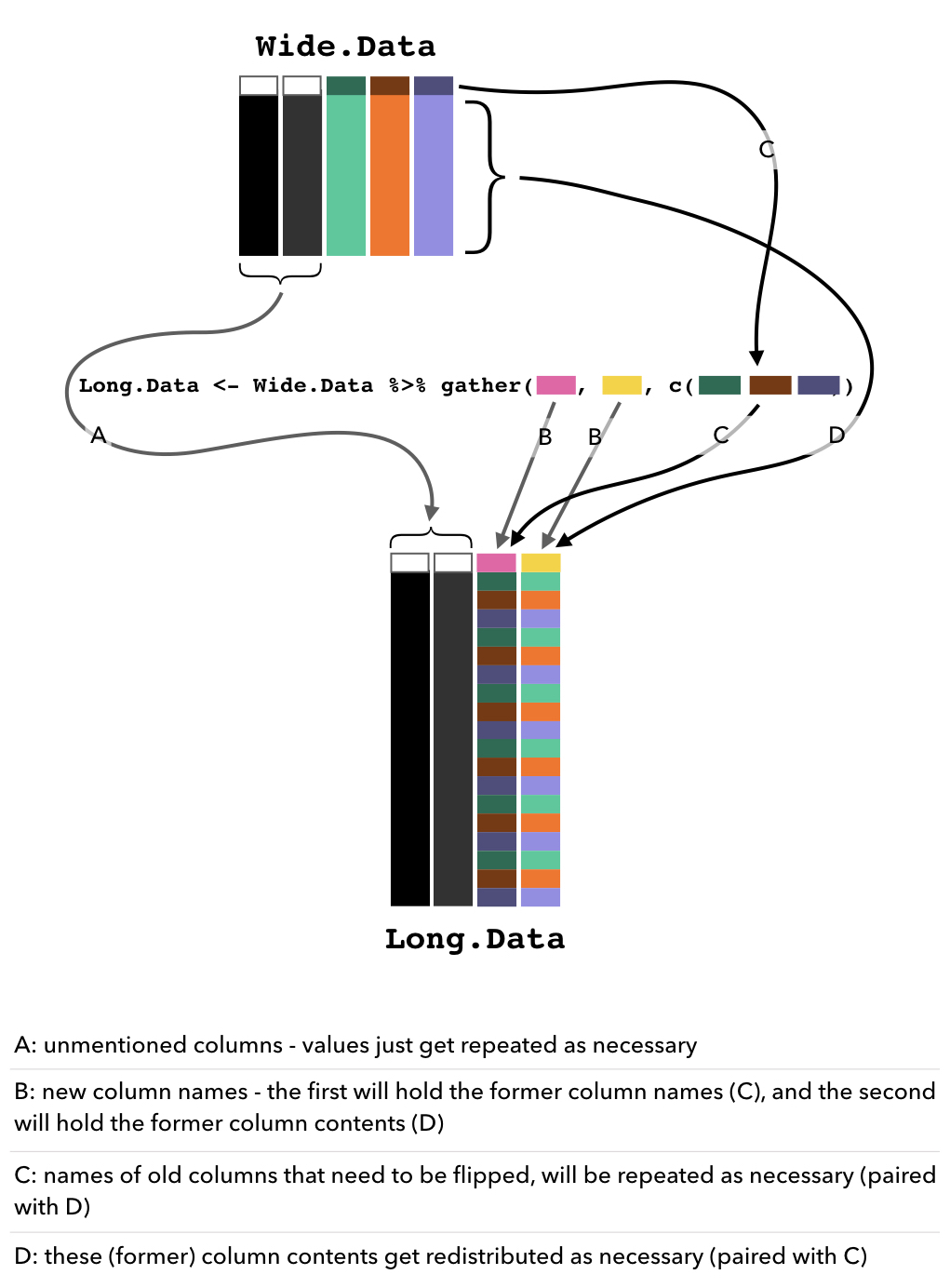
- I piped (
%>%) the original, wide form, data into thegatherfunction. - I gave it the new column names that I want: one name which will be the new column where the old column names are stored and repeated as necessary, and one name which will be the new column where all of the values from the old columns will be stored.
- I give it the indices of the columns that it should be rearranging.
Any unmentioned columns (in this example, Individual and ASclass) will keep their column names and the values within will just get repeated as necessary.
A desperate (and quite possibly, useless) attempt to represent this graphically:
Spread and Flop
Ok, so now let’s say we want to FLOP the data up into WIDE form - so, basically we want to do the opposite of what she just did above. We want to go from having one column per variable, to having only one row per orangutan - so we’d have one column for Individual, one column for ASclass, one column for each nest position (NestPos1 through to NestPos4), and the counts of each nest position will be in the respective columns.
I will use the spread() function from the tidyr package…
#SPREAD
data.wide <- data.long %>% spread(NestPosition, Counts)

#look at the whole thing
data.wide %>% print(n = Inf)
## # A tibble: 10 x 6
##    Individual ASclass          NestPos1 NestPos2 NestPos3 NestPos4
##    <chr>      <chr>               <dbl>    <dbl>    <dbl>    <dbl>
##  1 Boy        AdolescentMale         10       16        9       14
##  2 Englas     AdolescentMale          2        8       15       20
##  3 Jip        UnflangedMale           4       14        6        3
##  4 Loki       FlangedMale             8        8       18       13
##  5 Luaqlas    AdolescentFemale       12        6       11        7
##  6 Milo       AdolescentFemale       17        5       16        4
##  7 Mindy      AdultFemale            10       14        4       18
##  8 Monster    FlangedMale            11        8       11       20
##  9 Pi         AdultFemale             7       13       11       10
## 10 Roger      FlangedMale             6       18       15       19

str(data.wide)
## Classes 'tbl_df', 'tbl' and 'data.frame':    10 obs. of  6 variables:
##  $ Individual: chr  "Boy" "Englas" "Jip" "Loki" ...
##  $ ASclass   : chr  "AdolescentMale" "AdolescentMale" "UnflangedMale" "FlangedMale" ...
##  $ NestPos1  : num  10 2 4 8 12 17 10 11 7 6
##  $ NestPos2  : num  16 8 14 8 6 5 14 8 13 18
##  $ NestPos3  : num  9 15 6 18 11 16 4 11 11 15
##  $ NestPos4  : num  14 20 3 13 7 4 18 20 10 19
summary(data.wide)
##   Individual          ASclass             NestPos1        NestPos2
##  Length:10          Length:10          Min.   : 2.00   Min.   : 5.0
##  Class :character   Class :character   1st Qu.: 6.25   1st Qu.: 8.0
##  Mode  :character   Mode  :character   Median : 9.00   Median :10.5
##                                        Mean   : 8.70   Mean   :11.0
##                                        3rd Qu.:10.75   3rd Qu.:14.0
##                                        Max.   :17.00   Max.   :18.0
##     NestPos3       NestPos4
##  Min.   : 4.0   Min.   : 3.00
##  1st Qu.: 9.5   1st Qu.: 7.75
##  Median :11.0   Median :13.50
##  Mean   :11.6   Mean   :12.80
##  3rd Qu.:15.0   3rd Qu.:18.75
##  Max.   :18.0   Max.   :20.00
Again, it’s ridiculously simple:
- I piped (
%>%) the long form data into thespreadfunction. - I give it the name of the two columns that I want to be reorganized: the values from the first column will become the column names, and the values in the second column will be reorganized into those columns accordingly.
Any unmentioned columns (in this example, Individual and ASclass) will keep their column names and the values within will just get unduplicated as necessary.
That’s it. Easy Peasy once you get it to work. Inexplicably mind-boggling until then.